Computational Biomechanics

In FEAPpv as well as the full version of FEAP, you can write a Fortran subroutine to add a new constitutive model to the main program. Not only new constitutive models, you can also add a new element subroutine or even a new solver. To get started, you can study the built-in material models in FEAPpv. There are many examples of material models in FEAPpv. For example, the Neo-Hookean material model has been implemented in FEAPpv. You can download a copy of the FEAPpv source code online. The Neo-Hookean model as well as other material models are implemented in the subroutine elements\material.f.

The first step to implement your own material model in FEAPpv is to derive the Cauchy stress and elasticity tensors of your material model. Then, you can write a Fortran subroutine by using the material model interface available in FEAPpv. Once your user material model is ready, you can compile it together with the main FEAPpv program. The instruction to compile and build the FEAPpv executable file is described in the FEAPpv readme file. If you encountered an error saying that some .dll files such as libifcoremd.dll are missing while running the executable file for the first time on a Windows machine, please install the Intel Fortran Compiler Redistributable Libraries for your computer first.

As an example of the user material subroutine, the implementation of the Neo-Hookean hyperelastic material model in FEAPpv have been uploaded to the course repository together with a FEAPpv input file for the uniaxial extension test of a 2D rectangular model. Due to the limitation of FEAPpv, only the 2D mixed element is “available” (only partially, read below), it is not possible to test those user subroutines with 3D mixed elements in FEAPpv. Since we have already studied the analytical solution of a rectangular specimen under uniaxial test,

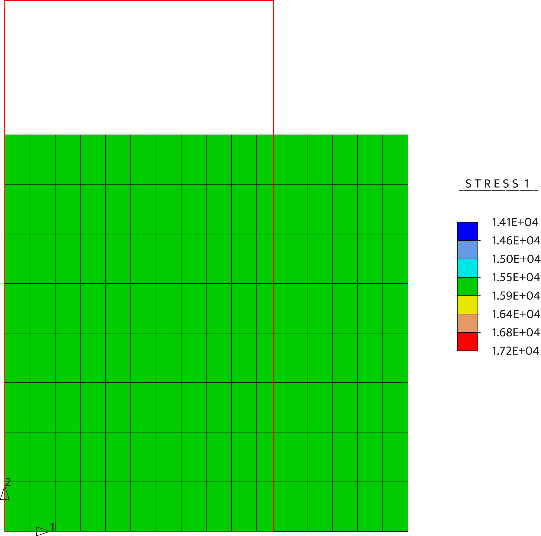
\[\sigma = \mu \left( \lambda^{2} - \lambda^{-1}\right),\]

where \(\lambda\) is the stretch in the loading direction. The following figure shows the initial (red frame) and deformed configurations of the rectangular model under uniaxial extension test up to a stretch of \(\lambda = 1.5\).

Here is a comparison of the computational solution by using FEAPpv with user subroutines and the analytical solution of the uniaxial extension test for \(\mu = 10\) kPa,

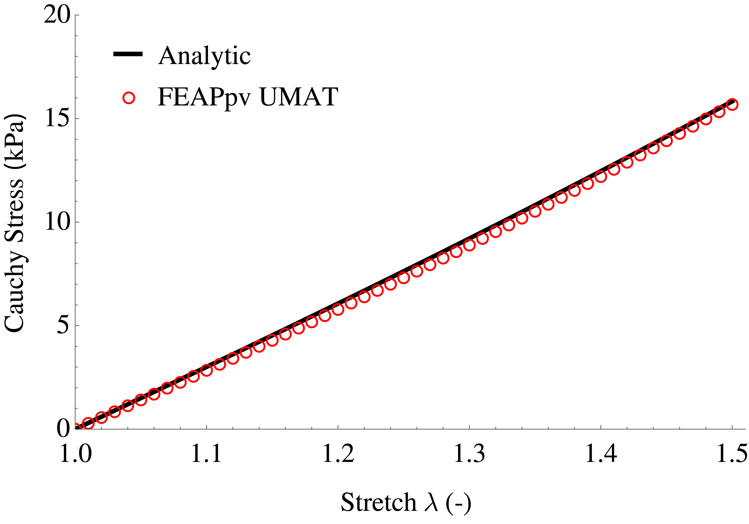
As shown, there is a small difference between the computational and analytical solutions. In fact, the total area of the deformed shape of the model is not equal to the total area of the model in the initial configuration. Thus, the material becomes compressible already. This is because the mixed 2D element in FEAPpv has not been completely implemented yet. The developers of FEAPpv are currently working to finish this implementation, and you may find it in a future release.

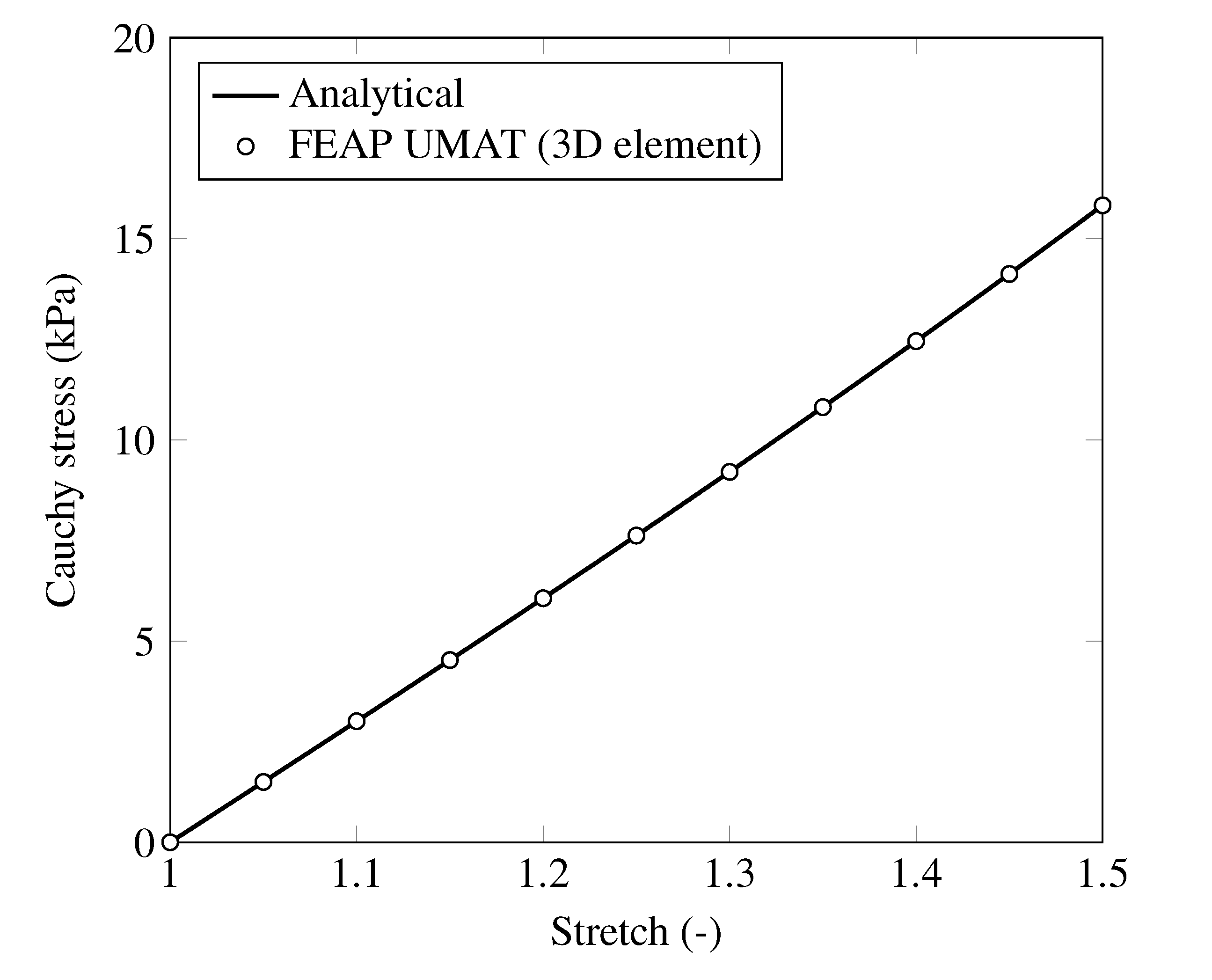
To make sure the user material subroutine is correct, a simple test with the 3D mixed elements in the full version of FEAP 8.5 (not FEAPpv because the 3D mixed element is not available in FEAPpv) shows exact match between the computational and analytical solutions.

The following figure shows the initial (red frame) and deformed configurations of the 3D model under uniaxial extension test up to a stretch of \(\lambda = 1.5\) with FEAP 8.5.

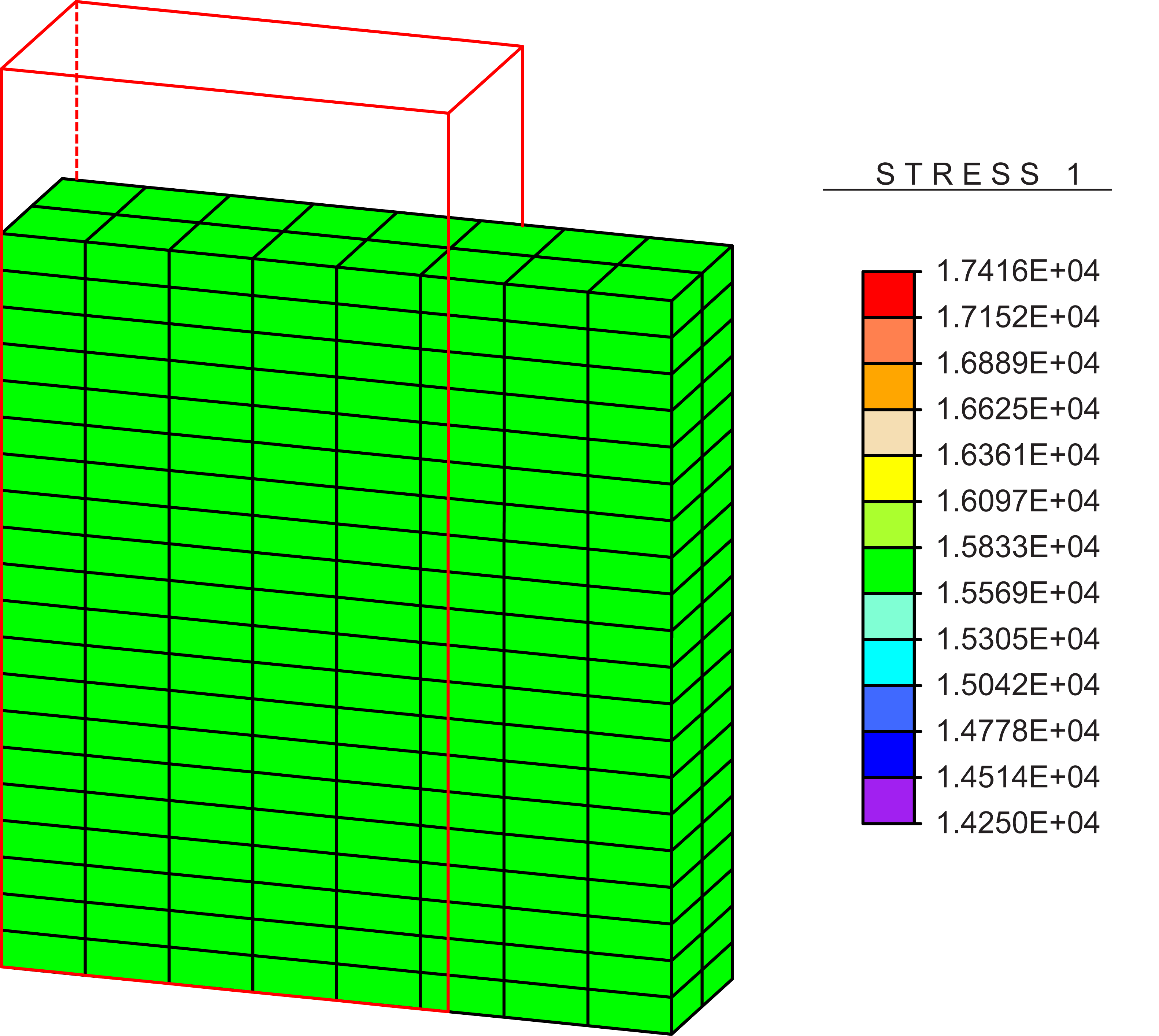
Note that the thickness of the model becomes smaller in the deformed configuration too.