Computational Biomechanics

Introduction

On May 21st, 2019, Wolfram Research, the company which created the Mathematica, launched the Free Wolfram Engine for Developers. The name Wolfram Engine may sound strange for some people. But it is the engine (kernel) behind the Mathematica. So all the programming features in Mathematica can also be used with this free Wolfram engine.

Licensing and Installation

To run the Wolfram Engine on your local machine, you need to request a free license, install the program, then activate the product. You will need to register a Wolfram ID to activate the Wolfram Engine. At first, download the Wolfram engine at http://www.wolfram.com/engine and install it according to the instruction online.

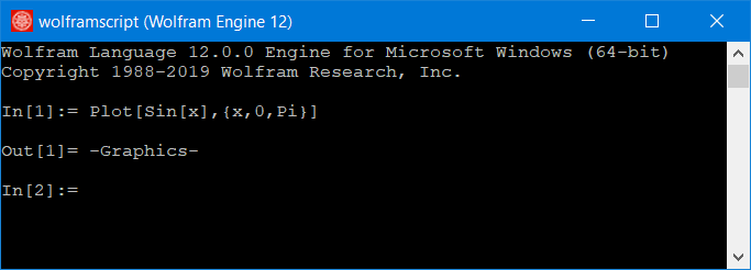
At this point, you should be able to run Wolfram Engine from your command line or terminal if you are using Linux or MacOS. However, the graphic output is not available on the command line.

Of course, you can use the built-in Export function to save the graphic to a file. But there is a second solution to make it display the graphic output. You can actually use the Wolfram Engine together with the Jupyter Notebook. At first, you need to install the Jupyter Notebook on your local machine according to the instruction online. If you have already installed Python on your machine, then you just need to run,

python -m pip install --upgrade pip
python -m pip install jupyter

Now, Jupyter Notebook is ready. Before you use it, you need to set a password for your Jupyter Notebook by running

jupyter notebook password

We need also to let Jupyter Notebook know about the Wolfram Engine. To do so, you need to first download the WolframLanguageForJupyter from its GitHub repository to your local hard drive. Then, unzipping the file will create a new folder, start a command line or Linux terminal in the newly created folder and run

configure-jupyter.wls add

Note that the file configure-jupyter.wls must be in that folder. If not, then you are in a wrong folder.

A Brief Tutorial of Wolfram Language with Jupyter Notebook

Once you have successfully added the Wolfram language interface to your Jupyter Notebook, then you can start Jupyter Notebook from command line by running

Jupyter Notebook

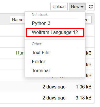
This command will invoke your default program to open a .html file. So make sure you are using Firefox or Google Chrome. Click New and then Wolfram Language 12 to create a new Wolfram notebook.

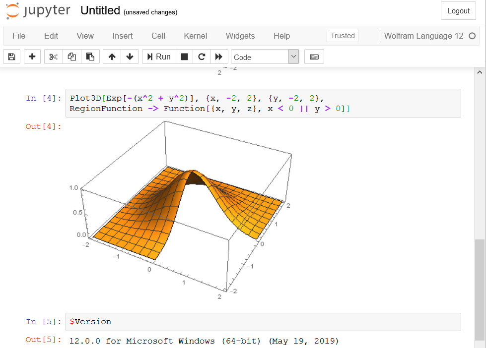
Then, you can use the Wolfram engine just as if it is Mathematica.

For example, the following code will plot the sine function from \(0\) to \(\pi\) and export the plot as a .svg file.

sineplot=Plot[Sin[x], {x, 0, Pi}]
Export["sineplot.svg", sineplot, ImageSize->300];

You can also export it to other file format such as .png or .pdf.

sineplot=Plot[Sin[x], {x, 0, Pi}]
Export["sineplot.png", sineplot, ImageSize->300];

Here is the output,

The Wolfram notebook file (a .ipynb file) as well as the exported picture file you created in Jupyter Notebook will be located in the folder where you initialized the Jupyter Notebook (the folder where you started the Jupyter Notebook from the command line).

It is also possible to plot complicated functions such as,

sincplot=Plot3D[Sinc[Sqrt[x^2-x*y+x+y^2-y]], {x,-10,10},
{y,-10,10}, PlotRange->{Full,Full,{-1,1.5}},Mesh->60, 
ColorFunction -> Hue] 
Export["sincplot.svg", sincplot, ImageSize->450];

Here is the output,

It seems the resolution of the .svg image is not very high. Here is the PDF output with the same code.

sincplot=Plot3D[Sinc[Sqrt[x^2-x*y+x+y^2-y]], {x,-10,10},
{y,-10,10}, PlotRange->{Full,Full,{-1,1.5}},Mesh->60, 
ColorFunction -> Hue] 
Export["sincplot.pdf", sincplot, ImageSize->450];

Wolfram Script Example

It is also possible to write a script in Wolfram Language and run it from the command line. You can find an example here. Download the raw file (.wls file) of that example and run it in your command line or terminal as,

.\SolveHeatEquation.wls

Here is the output in PDF, and see also the following figure,

You can find more information about the script of Wolfram language here.